CS131 Notebook

A individual notebook for cs131: computer vision Chapter1-4(relating to pdf 2, 4 ,5, 6)

More blogs or fun,see xiaoxin83121

Chapter1: Pixels and Filters

Color

Color: The result of interaction between physical light in the environment and our visual system. **
It’s a **psychological propety of our visual experiences, NOT physical property.

Color Space

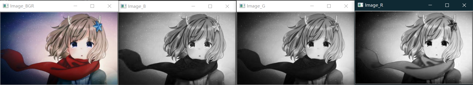
RGB Cubic color space

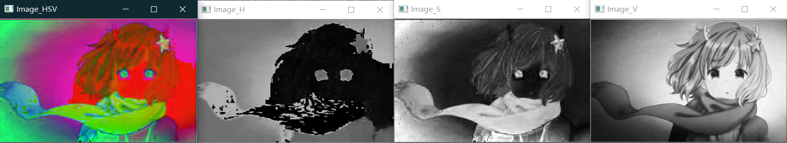
HSV(Hue, Saturation, Value: 色调，饱和度，明度): cone

img = cv2.imread("./test.jpg") # BGR==0:b, 1:g, 2:r
img_hsv = cv2.cvtColor(img, cv2.COLOR_BGR2HSV)
img_grey = cv2.cvtColor(img, cv2.COLOR_BGR2GRAY)
img_b = img[..., 0]
img_g = img[..., 1]
img_r = img[..., 2]
cv2.imshow("Image_B", img_b)
cv2.imshow("Image_G", img_g)
cv2.imshow("Image_R", img_r)
cv2.imshow("Image_BGR", img)

Image sampling and quantization

Resolution: sampling parameter, defined in dots per inch(DPI) or spatial pixel density.
An image contains discrete number of pixels: a matrix or a set of matrix(r,g,b,etc.)

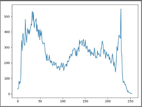
Image histograms

provide the frequency of the brightness(intensity) value.

img = cv2.imread('./test.jpg')
    img = cv2.cvtColor(img, cv2.COLOR_BGR2GRAY)
    h = np.zeros(255)
    for row in range(img.shape[0]):
        for col in range(img.shape[1]):
            h[img[row, col]] += 1
    plt.plot(h)
    plt.show()

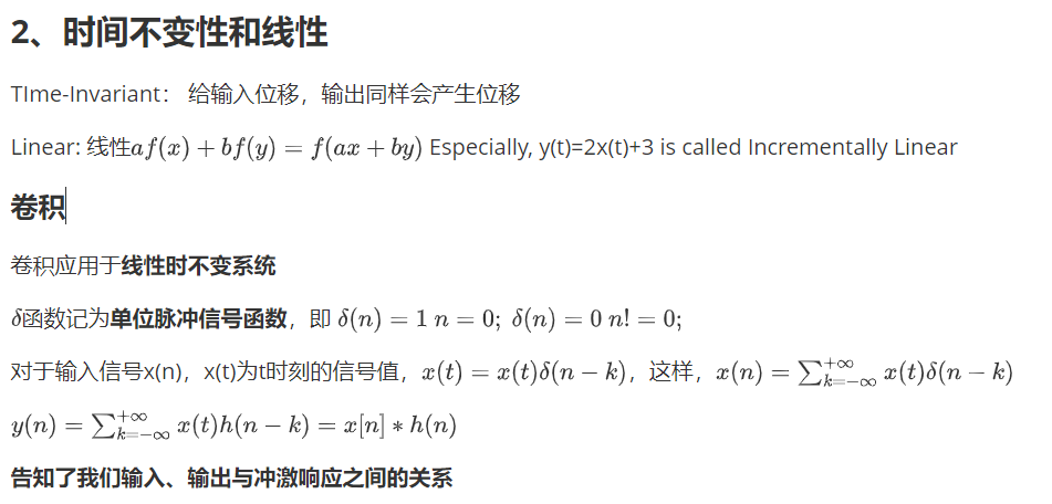
Linear systems(filter)

Filtering: Forming a new image whose pixel values are transformed from original pixel values. (两个矩阵之间的线性变换)
详细内容可以查看信号与系统中关于Linear shift invariant system的详细描述,这里截取自我个人的note

Convolution手动实现：

def convolution_filter(stride=1):
    # manually convolution and see how it changes
    img = cv2.imread('./test_high.jpg')
    img = cv2.cvtColor(img, cv2.COLOR_BGR2GRAY)
    # generate kernel
    kernel = np.ones((3, 3)) / 9
    # kernel = np.array([[0, 1, 2], [0, 1, 2], [0, 1, 2]]) / 9
    # generate output feature map
    output = np.zeros_like(img)
    time_before = time.time()
    for row in range(0, img.shape[0]-2, stride):
        for col in range(0, img.shape[1]-2, stride):
            mat = img[row:row+3, col:col+3] * kernel
            val = np.sum(mat.flatten())
            try:
                output[int(row/stride) + 1][int(col/stride) + 1] = val
            except:
                print('error happened when row={},col={}'.format(row, col))

    time_after = time.time()
    print("time consume={}".format(time_after- time_before))

    cv2.imshow("origin", img)
    cv2.imshow("convolution", output)
    cv2.waitKey()
    cv2.destroyAllWindows()

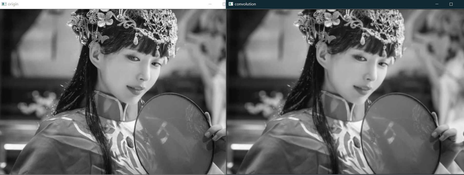
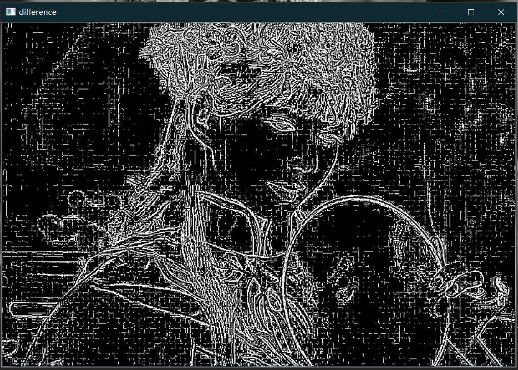
右图变糊了一点，实际测试[[0,1,2],[0,1,2],[0,1,2]]/9的卷积核差距不大，stride的调整也不会对整体观感有明显影响， origin file和convolution的结果之间的difference(Difference of Gaussian, DoG，chapter-4会使用到)的结果如下：

Chapter2: edges

Edges typically occur on the bondary between two different regions in an image.

edge detection

Identify sudden changes(discontinuities) in an image. with Good detection, Good localization, Single response

Image Gradient

1D discrete derivative filters As we all know,
backward filter: $f(x)-f(x-1)=f’(x)$, with a vector [0, 1, -1]
forward: $f(x)-f(x+1)=f’(x)$, with [-1, 1, 0]
central: $f(x+1)-f(x-1)=f’(x)$, with [1, 0, -1 ]
vector means : [f(x+1), f(x), f(x-1)], is that clear?
2D discrete derivate filters:

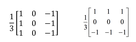
Left kernel means gradient in x-axis, result as below:

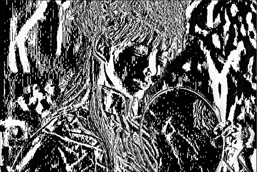
Right kernel means gradient in y-axis, result as below:

显然，各自保存了x方向上和y方向上的离散梯度变化。

Other kernel like: $[[1, 0, -1], [2, 0, -2], [1, 0, -1]]=[1, 2, 1]^{T}[1, 0, -1]$. 为高斯核与梯度核的结合体(x, y derivatives of Gaussian)。

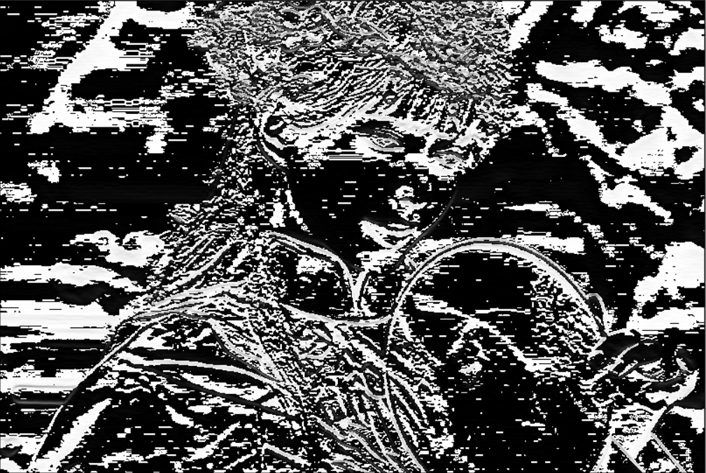
Canny edge detection

Filter image with x,y derivatives of Gaussian
Find magnitude and orientation of gradient
Non-maximum suppression(Single response)

Define low and high thresholding

edge_output = cv2.Canny(img, 50, 100) # wheels of opencv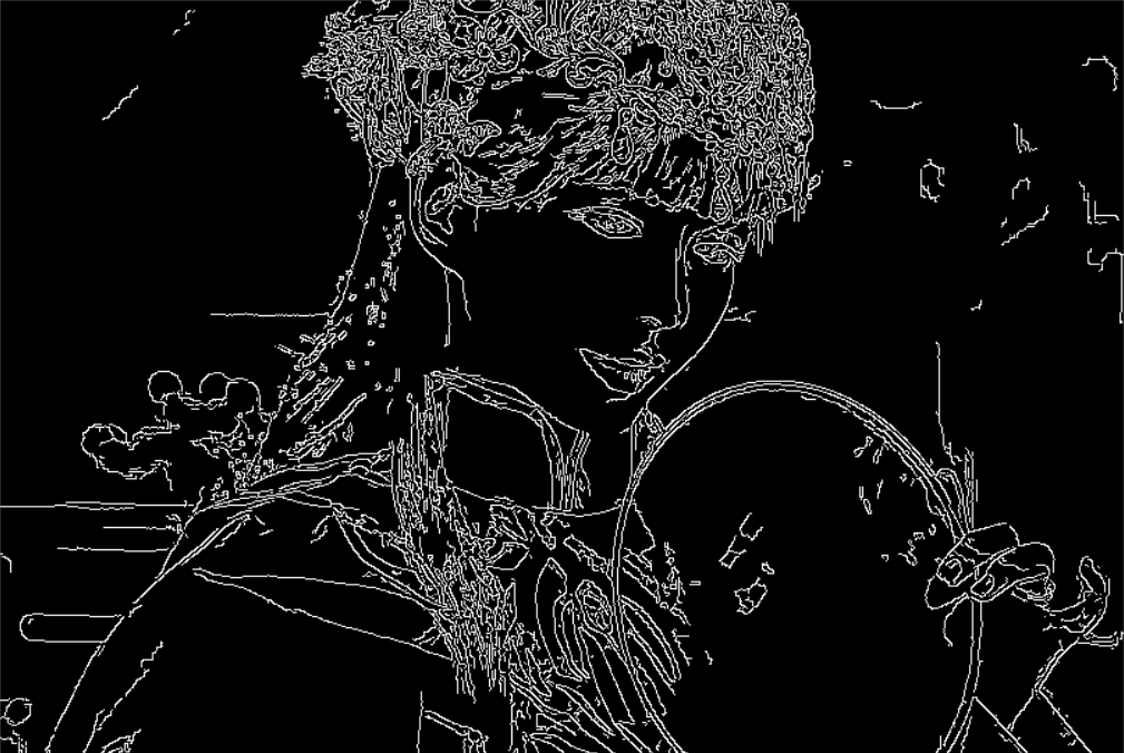

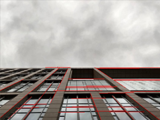
Hough transform

$y=ax+b$，This is the simplest statement of line with certain $a$ and $b$,
But we can also get $b = -ax+y$ with certain $x$ and $y$
for $(x_{1}, y_{1})$ and $(x_{2},y_{2})$, there will be two lines in $a\&b$ space with intersection of $(a^{‘},b^{‘})$. Convert it to $x\&y$ space, line is determined.

img = cv2.imread('./test_ver_hor.jpg')
img_grey = cv2.cvtColor(img, cv2.COLOR_BGR2GRAY)
edges = cv2.Canny(img_grey, 50, 100)
lines = cv2.HoughLinesP(edges, 1, np.pi/180, 30, minLineLength=60, maxLineGap=5)
lines = lines[:, 0, :]
for x1, y1, x2, y2 in lines: # 画出红线不能在grey上画噢
    cv2.line(img, (x1, y1), (x2, y2), (0, 0, 255), 1)
cv2.imshow("Hough", img) 
cv2.waitKey()
cv2.destroyAllWindows()

Chapter3：RANSAC and feature detectors

RANSAC: RANdom SAmple Consensus

inliers: 内点，在某个拟合区域内的样本点；

outliers: 外点，在拟合区域外的样本点，干扰项；

核心思想：不断随机生成拟合区域样本，选择拟合区域内内点最多的样本；投票策略。 eg: 拟合直线，随机选取两点定一条直线，距离这条直线距离d以内的点都为inliers；

Local invariant features

和SIFT类似, 在Chapter-4继续

Harris Detector

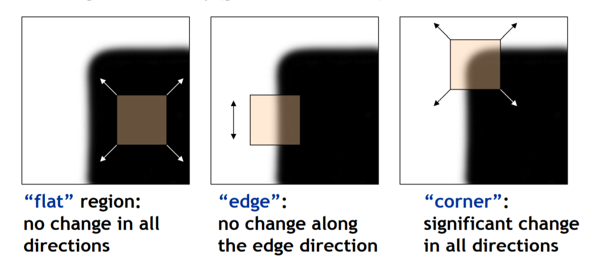
利用窗口再在不同方向上的移动上的梯度变化来感知边缘和边角；问题的关键是如何量化？
假设$u$和$v$是$x$和$y$方向上的移动距离，那么intensity difference可以量化为$I(x+u, y+v) - I(x, y)$
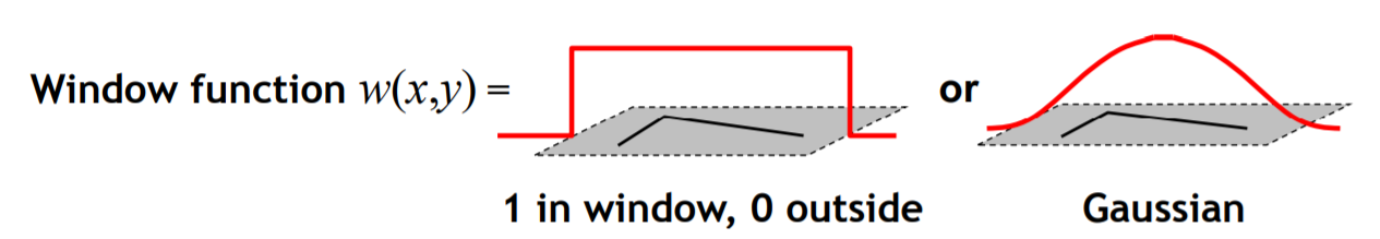
So，we can get Harris Detector Formulation: $E(u,v)=\sum_{x,y}w(x,y)[I(x+u, y+v) - I(x, y)]^{2}$
$w$ is windows function, belowing two are often used:

By taylor expansion, we can get $I(x+u, y+v) - I(x, y) \approx I_{x}u+I_{y}v$
So, the Harris Detector Fomulation can be written as:
$E(u, v) \approx \begin{bmatrix} u & v \end{bmatrix} \space \sum_{x,y}w(x, y) \begin{bmatrix} I_{x}^{2} & I_{x}I_{y} \\ I_{x}I_{y} & I_{y}^{2} \end{bmatrix} \space \begin{bmatrix} u \\ v \end{bmatrix} =w(x, y) \space R^{-1} \begin{bmatrix} \sum{I_{x}^{2}} & \sum{I_{x}I_{y}} \\ \sum{I_{x}I_{y}} & \sum{I_{y}^{2}} \end{bmatrix} R, as \space R= \begin{bmatrix} u \\ v \end{bmatrix}$

我们记

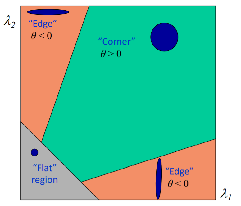
$M = \begin{bmatrix} \sum{I_{x}^{2}} & \sum{I_{x}I_{y}} \\ \sum{I_{x}I_{y}} & \sum{I_{y}^{2}} \end{bmatrix}$ 由实对称矩阵的性质可得， $M = R^{-1} \begin{bmatrix} \lambda_{1} & 0\\ 0 & \lambda_{2} \end{bmatrix} R$ 经过转化后，$E(u, v)$随着$u$和$v$变动的幅度就由矩阵$M$中的参数$\lambda_{1}$与$\lambda_{2}$来决定，若$\lambda_{1}$大，那么$E(u, v)$随着$u$变动幅度也大……
因此当$\lambda_{1}»\lambda_{2}$或者$\lambda_{2}»\lambda_{1}$, 判定为edge；
$\lambda_{1} \approx \lambda_{2}$并且两个值都很大，判定为corner；
$\lambda_{1}$和$\lambda_{2}$都比较小，判定为flat;
这样的判定法不够方便，记$\theta=det(M)-\alpha trace(M)^{2}=\lambda_{1}\lambda_{2}-\alpha(\lambda_{1}+\lambda_{2})^{2}, \alpha=0.04 \space to \space 0.06$

thus,

Wonderful! Now, Let’s summarize the Harris Detection:

calculate Image derivatives, $I_{x}$ and $I_{y}$
calculate square of derivatives, $I_{x}I_{y}$, $I_{x}^{2}$ and $I_{y}^{2}$
apply Gaussian filter or other windows function
calculate $\theta$ , get corner collection
apply Non-maximum suppression

Chapter4: Feature Descriptors

After extract Ket point in Chapter3， There is another question: What will happen if scale or orientation changes? How to match the same key points in another image with different scales and orientation?

Scale invariant detection:

Harris-Laplacian

Find local Maximum of :

Harris corner detector in Space
Laplacian in Scale

SIFT

Find local Maximum of: Difference of Gaussian filter in Space and Scale Algorithm are as follows: For a SIFT descriptor,

rotate image gradient in a calculated $\theta$; $L(x,y)$为Gaussian Smoothed Image的pixel value.

$\theta(x,y)=tan^{-1}(\frac{L(x, y+1)-L(x, y-1)}{L(x+1,y)-L(x-1,y)})$

split SIFT descritor as $4 \times 4$ histogram array, in each histogram, split 8 orientation bins .

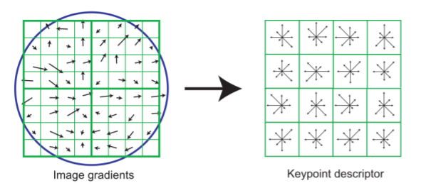
use the array with $4 \times 4 \times 8$ to match.

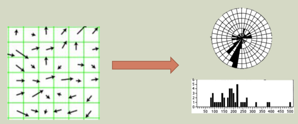
HOG: Histogram of Oriented Gradients

一言以蔽之：对整图(SIFT针对descriptor)分cell使用histogram记录梯度变化，后续利用分类器分类

What’s More, Resizing, segmentation, and cluster , See cs131_2

xiaoxin83121.github.io

Blog