Object Detection

YOLO

YOLO(You Only Look Once) one stage algorithm. This blog will introduce four edition of YOLO network.

YOLO v1

A single convolutional network simultaneously predicts multiple bounding boxes and class probabilities for those boxes.

优点：

1. extremely fast；
2. reasons globally about the image when making predictions.
3. learns generalizable representations of objects.(egs: train with natural images and test with art-work)

缺点：

1. one grid only generate 2 bounding box for a single class, leading to negative to small object
2. small error on small bbox has a great effect on IOU.

结构：

• Unified Detection: predicts all bounding boxes across all classes for an image
• grid: devide the whole image into $S \times S$ grid, each grid predicts B bounding boxes and confidence scores. bounding boxes consists of 5 elements(Total $B \times 5$): center points x and y relative to the bounds of the grid cell; box width and height w and h relative to the whole image; confidence relative to the IOU between the predicted boxes and ground truth, which in equations: $Pr(Object) \times IOU_{pred}^{truth}$

• Instead: grid predicts C Probability of $Pr(Class_{i}

  Obejct)$

• So we can get $Pr(Class_{i}) \times IOU_{pred}^{truth}$ from the upper two equations
• summary: We get a output of $S \times S \times (B \times 5 + C)$tensor(egs: S=7, B=2, C=20 when dataset is pascalvoc)
• 与论文Real-time Grasp Detection Using Convolutional Neural Networks中的方法类似–都是Joseph Redmon写的

trick on training

• penalty of incorrect classification
• leaky ReLu(Rectified Linear activation)
• dropout layers to avoid overfitting

experiment methods

• error analysis: seperate predictions as correct, localization, background, etc. 本质上是一个召回率计算过程的细化，不单分false or positive; YOLO具有higher localization errors but lower background errors.
• combine Fast Rcnn with YOLO seperately to boost results 验证了YOLO在去除background类别的有效性；Fast+YOLO， Fast+Fast VGG等对比实验，说明优化不是由combination带来的

YOLO9000: YOLO v2

优化

• Batch Normalization: lead to 2% improvement in mAP; with BN, network can remove dropout without overfitting.
• high-resolution classifier
• anchor-boxes: From Faster-RCNN and user cluster instead of hand pick priors. Though Redmon introduce it a lot, the latest version didn’t use it.
• Direct location prediction: 使用了anchor-boxes后，bounding boxes会在整个图里随机生成，在训练一开始会极不稳定； Solution: Use relative offset from grid cells.
• Multi-scale Training: Since YOLO use convolutional and pooling layers, the input could be different sizes during training.
• new classification network: Darknet-19, 19 convolutional and 5 maxpooling layers.
• Hierarchical classification: Using Wordtree, a category tree. To calculate a leaf node’s probability, condition probability from root to node should be recorded.

实验

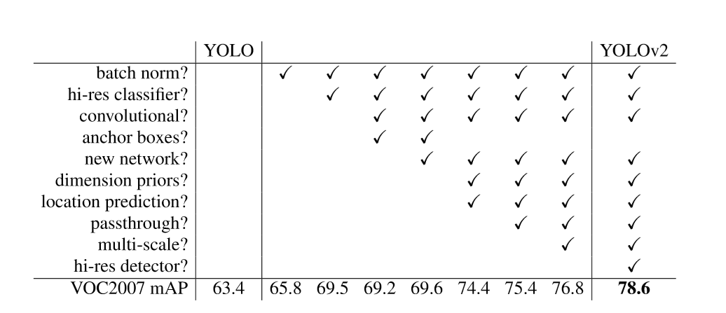
This is a experiment record picture with variance and mAP results. It is Impresive. But we can see that anchor-boxes is ignored in formal YOLOv2. Weird.

YOLOv3

most of methods have been put in yolov2, yolov3 is more stronger and caters to bussiness.

进步

• multiscale: yolov3 predicts boxes at 3 different scales and each grid predicts 3 boxes in certain scale. Small objects are better.
• optional backbone network: Darknet-19, Darknet-53, etc.
• Things that didn’t work: Anchor boxes instability as yolov2; Focal loss; Dual IOU thresholds like .3 and .7, but .5 is good

code

• Written in C…
• The installation is quite simple. Use command make in the source root to compile. Then download yolov3.weights to source root. Run command ./darknet detect cfg/yolov3.cfg yolov3.weights data/dog.jpg . If this command give you error information like file not found or first must be [net], you need to change file format using dos2unix.exe in windows, and add one line code which could be found in issues to src/parse.c
• todo

YOLOv4

published in 2020 without Redmon, but improve a lot

要点

• generally speaking, yolo v4 take several periods in object-detection like pre-process, network architecture, post-process, etc.
• The research method is similar with YOLO v2, but more sufficient.
• Finally YOLOv4 choose SPP(Spatial Pyramid Pooling)、modified SAM(Spatial Attention Module) and modified PAN(Path Aggregation Network). Many methods processing dataset and different Loss function like GIOU are used and verified in experiment.

SSD

Single Shot MultiBox Detector

要点

• Multi-scale feature maps for detection: convolutional feature layers decrease progressively.
• Convolutional predictors for detection: Compared to YOLO, SSD use convolutional layers without using fully-connection layers
• Default Box and aspect ratios: “The default boxes tile the feature map in a convolutional manner, so that the position of each box relative to its corresponding cell is fixed.”

  There is $m \times n$ feature map, which means $m \times n$ cells. Each cell relates to a given location, which has k boxes. So, there are $kmn$ boxes. And each box relates to the outputs of the sum of classification numbers and 4 offsets. So, there are $(c+4)$ outputs per box. Finally, There will be $(c+4)kmn$ outputs per feature map whose shape is $m \times n$.

训练

MultiBox: focus on generating class-agnostic bounding boxes in regression method. Loss-function: $F_{match}(x,l)$ is a L2 Loss and $F_{conf}(x,c)$ is a Binary Entropy Loss. And $x_{ij}$means i-th prediction matches to j-th true object. $F(x,l,c)=\alpha F_{match}(x,l) + F_{conf}(x,c)$ especially, $\alpha$ set to 0.3

• Matching Strategy: Match GT to default box with best Jaccard Similarity(Instead of MultiBox：Pick higher scores rather than maximun overlap)
• Loss Function: $L=\frac{1}{N}(L_{conf}+\alpha L_{loc})$ $L_{conf}$ –> softmax loss; $L_{loc}$ –> $ smooth_{L1}$
• Choose different scales and aspect ratios: Like R-CNN, SSD determine default boxes in certain feature map by two parameters $\alpha_{r}$ and $s_{k}$
  $\alpha_{r}={1,2,3,\frac{1}{2}, \frac{1}{3} }$ And $s_{k}=s_{min}+\frac{s_{max}-s_{min}}{m-1} (k-1)$

  for k in range(m):
    for a in ar:
        if a==1:
            _sk = sqrt(s_k*s_k+1)
            r1 = (s_k*sqrt(a), s_k/sqrt(a))
            r2 = (_sk*sqrt(a), _sk/sqrt(a))
        else:
            r = (s_k*sqrt(a), s_k/sqrt(a))
  # there will be 6 default boxes per feature map location
  

实验

• Data augumentation is crucial！
• More default box shapes is Better！
• atrous convolution is Better: 空洞卷积，卷积操作并非对连续像素进行操作，而是隔着某个参数=k(1,2,…)进行卷积；
• Multiple output layer at different resolutions is Better

Heatmap

以Center-Net为例

该模型对于输入图像首先进行了预处理，包括图像仿射变换、大小调整等。对于训练数据，对原始图像进行预处 理的同时，需要对标注的检测框应用高斯模糊算法得到种类热度图，在训练过程中，以 多种不同的中枢网络（主要包括沙漏网络 (Stacked Hourglass Net)、ResNet、DCN网络等）为基础，适用于不同的目标检测任务，如人体姿态检测、3D 检测与平面检测 等。训练过程中，分别计算热度图的损失函数、长宽损失函数、偏移值损失函数和总损 失函数，用以网络训练的收敛与优化。

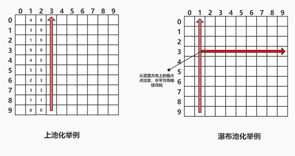
对于测试数据，经过预处理并加入到检测网络得到热度图等信息之后，需要进行解 码与处理。处理的过程主要是针对热度图应用 NMS算法，和中心池化 (Center Pooling) 与瀑布池化 (Cascade Corner Pooling) 两种池化操作。NMS算法为诸多目标检测网络公 用的去除冗余检测框的方法，在此不再赘述。中心池化和瀑布池化是从 Corner Net网络提出的边缘池化的改进版，在 Corner Net 中，边缘池化的作用是通过与贝叶斯公式类似的先验概率验证方式，通过既有概率来推断边界框中的四个端点。边缘池化共分为上、 下、左、右四个方向池化，以上-左池化为例，上池化操作从下至上搜索最大值，选取扫 描过程中已经遇到的最大值与当前值中的最大值写入当前值，左池化操作为从右至左， 扫描过程相同。得到上池化与左池化后的特征图后，将两个特征图按元素相加，得到的新的特征图用于预测热度图以及偏移等任务。